In this tutorial, we will perform a geometry optimization of an organic compound (a nematic liquid crystal) using Gaussian16.
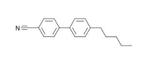
Molecular structure of the compound we will be calculating.
Step 1: generate a Gaussian input file
We begin with an approximate geometry for the organic compound, retrieved from a database, obtained from XRD data, or built in a molecular structure program; in any case, we start with a file detailing the type and position of the atoms in the molecule. In this tutorial, we will use this file in XYZ format.
The next step is to generate a Gaussian input file. This can be done by hand, using GaussView, or using extensions in other molecular visualization programs. We will use nematic.com:
%NProcShared=4
#t B3LYP/6-311G(d,p) Opt

Nematic

0 1
N    2.08964    6.18040    -0.54103
C    2.37488    5.07973    -0.49334
C    2.03482    3.68239    -0.38365
C    1.95525    3.07404     0.86340
C    1.62472    1.72435     0.96946
C    1.36382    0.93515    -0.16783
(...)
H   -4.90370   -8.18710     0.08922
H   -3.53507   -8.45230     1.18121
- Line 1: instructs Gaussian to use 4 processors in a single node for our calculation.
- Line 2: provides the Gaussian route, i.e. the instruction specifying the calculation(s) to be performed.
- #t indicates terse output, producing a leaner output file.
- B3LYP/6-31G indicates the type of calculation (DFT hybrid functional B3LYP) and the basis set (6-31G) to be used.
- Opt specifies a geometry optimisation calculation.
- Line 4: contains the calculation title.
- Line 6: specifies charge and multiplicity.
- Lines 7-15: starting-point geometry, in XYZ format. Each line corresponds to a new atom, indicating atom type and coordinates.
Remember!
For more information, please check Gaussian documentation .
Step 2: prepare a shell script
In order to submit the job, we need to compose a shell script including module preparation and the Gaussian command. We will use the script nematic.slm:
#!/bin/bash
#SBATCH -J nematic
#SBATCH -e nematic.err
#SBATCH -o nematic.log
#SBATCH -n 1
#SBATCH -c 4

module load apps/gaussian/g16b1

INPUT_DIR=$SLURM_SUBMIT_DIR
OUTPUT_DIR=$SLURM_SUBMIT_DIR
INPUT_FILE=nematic.com
OUTPUT_FILE=nematic.out

date
cp -r $INPUT_DIR/$INPUT_FILE $SCRATCH
cd $SCRATCH
srun g16 < $INPUT_FILE > $OUTPUT_FILE
cp ./* $OUTPUT_DIR
date
A brief reminder of SLURM files structure:
- Line 1: Must be present to identify the file as a bash script.
- Line 2: Defines the job name in the SLURM system.
- Line 3: Instructs SLURM to send standard output from the job to a file.
- Line 4: Instructs SLURM to send error output from the job to a file.
- Line 5: Gaussian uses OMP for paralelization. Always use 1 task.
- Line 6: Requests 4 cores for the job. Number of threads per task.
- Line 8: Load the required modules.
- Line 10 and 13: Defines the input's and output's directories and files.
- Lines 15 and 20: Print current time (starting and end respectively).
- Line 16: Copy the input file from your home to $SCRATCH; make sure you have uploaded the input file to your chosen path (INPUT_DIR) before running the script.
- Line 17: Move to the temporary (local disk) directory, defined by the variable $SCRATCH; I/O is more efficient when run on $SCRATCH.
- Line 18: This is the line that actually launches the calculation.
- For Gaussian16, command syntax is: g16 < [input file] > [output file].
- Line 19: Copy the output file back from $SCRATCH to your home (OUTPUT_DIR).
Step 3: upload the files to the server
We need to upload the shell script and Gaussian input files onto the HPC storage. From our local directory holding the files, we call this command:
scp -P 2122 nematic.com nematic.slm youruser@hpc.csuc.cat:/home/youruser/
If you want to send the files to a different path, just make sure you create the appropriate directory in advance. This path should match the cd instruction in your SLURM script.
scp -P 2122 [input file(s)] youruser@hpc.csuc.cat:/home/youruser/your_chosen_path/
You can also use sftp to manage uploads and downloads. Remember to use port 2122 to secure connect to our machines.
Step 4: launch and monitor the job
To launch the job, we remotely log in to the HPC facilities (If we have not done it already). For more information about how to connect to the cluster, follow the instructions of How to connect to Pirineus and Canigó:
We will arrive at our /home/youruser/ directory. If we have uploaded the files to a different directory, we should move to it.
cd /your_chosen_path/
To launch the job, we send the nematic.slm script to sbatch:
sbatch nematic.slm
SLURM will automatically send the job to a queue that meets its requirements.
For an overview of the queues and their limitations:
sinfo
To check on the job status:
squeue
The output of this command looks like this:
JOBID	PARTITION		NAME		USER	ST		TIME	NODES	NODELIST(REASON)
 1933         std 	 nematic   user_name	 R   1:40:15      	1 	pirineus1
- JOBID indicates the number that identifies the job in the SLURM system.
- PARTITION the queue where the job has been submited.
- NAME is the label we provided with SBATCH -J in the script.
- USER is the user who submitted the job.
- ST indicates job status, for example PD (pending), R (running), etc.
- TIME is the job execution time.
- NODES is the number of nodes used for the job.
- NODELIST(REASON) indicates the node name where the job is executed. If the job is pending, indicates the reason why it is pending.
We can cancel a pending or running job:
scancel yourJOBID
Step 5: retrieve the results
We can add the line "#SBATCH --mail-user=user@mail.com" to our slm file to receive an email notification when the job is complete.
To retrieve the output file, we run this command in terminal (from the local directory where we want to download the files):
scp -P 2122 youruser@hpc.csuc.cat:/home/youruser/your_chosen_path/nematic.out .
The nematic.out file will contain the full output of our Gaussian calculation. GaussView provides a practical GUI to analyse the results, but all of the information is accessible in the text file. For instance, running the command
cat nematic.out | grep -A1 'Dipole moment'
will return the dipole moments of the initial and final (optimized) geometries, while the command
cat nematic.out | grep 'SCF Done' | cut -c12-
will print the total energy after each step of geometric optimisation.
The final, optimised geometry, in XYZ format, should be very similar to this one.