In this tutorial, we will perform a molecular dynamics simulation of a protein (Esculentin-1A, from Pelophylax esculentus) using Gromacs version 2018.1.
| Table of Contents | ||
|---|---|---|
|
| Tip |
|---|
Apart from the actual molecular dynamics program, Gromacs contains a long list of specific tools for the preparation, analysis and post-processing of MD simulations. Since it is open source software, it is highly advisable to install Gromacs in your local machine to perform these auxiliary operations. |
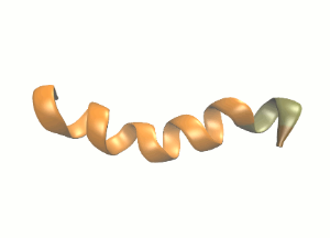
Schematic secondary structure of the protein we will be simulating.
Step 1: generate the Gromacs input files
We start by downloading the pdb file from the RCSB Protein Data Bank. This file format, designed for peptides, contains the aminoacid sequence of esculentin and additional structural information. However, this format differs from Gromacs structure inputs. We will use the Gromacs tool pdb2gmx to convert the file to Gromacs-readable format.
In our local machine, we move to a directory containing the pdb file and type:
| Code Block | ||
|---|---|---|
| ||
gmx pdb2gmx -f 2n6m.pdb -o esculentin.gro -p esculentin.top -ignh |
Since we haven't specified the force field or water model, the program will demand these interactively. We will choose GROMOS96 54a7 as the force field and the less accurate but inexpensive SPC water model. We have also instructed pdb2gmx to ignore hydrogen atoms in the pdb file (-ignh option). More information about gmx pdb2gmx here.
This command will generate three files in the current directory.
Structure file (.gro)
| Code Block | ||||||
|---|---|---|---|---|---|---|
| ||||||
ESCULENTIN-1A
  201
    1GLY      N    1   0.133   0.000   0.000
    1GLY     H1    2   0.118  -0.094   0.030
    1GLY     H2    3   0.185   0.049   0.070
    1GLY     H3    4   0.045   0.045  -0.014
    1GLY     CA    5   0.207   0.000  -0.125
    1GLY      C    6   0.234   0.140  -0.176
    1GLY      O    7   0.196   0.174  -0.288
    2ILE      N    8   0.300   0.221  -0.094
    2ILE      H    9   0.328   0.188  -0.004
    2ILE     CA   10   0.332   0.359  -0.132
(...)
   21GLY      C  199  -1.436   0.231  -2.356
   21GLY     O1  200  -1.539   0.169  -2.328
   21GLY     O2  201  -1.386   0.228  -2.482
0.10000 0.10000 0.10000 |
The structure file contains information about the atoms that conform the system we are simulating.
- Line 1: contains the system name.
- Line 2: contains the total number of atoms in the file (must match the actual number of lines).
- Lines 3-16: each line corresponds to one atom in the system, containing the following information (left to right):
- Residue number and type (for instance, the first residue in the file is glycine).
- Atom type. If more than one atom of the same type is present in a residue, these are also consecutively numbered.
- Atom number.
- Coordinates of the atom, XYZ, in nm.
- Line 17: contains the simulation box size, in nm.
More information about the .gro file can be found here.
Topology file (.top)
Include topology file (.itp)
| Code Block | ||||||
|---|---|---|---|---|---|---|
| ||||||
[ position_restraints ]
     1     1  1000  1000  1000
     5     1  1000  1000  1000
     6     1  1000  1000  1000
     7     1  1000  1000  1000
(...) |
Include topology files are auxiliary files containing additional topology information. They can be called into the main topology file via the #include mechanism, thus allowing for a modular approach to topology definitions (for instance, for special solvent parameters). File format is identical to .top files.
In our case, pdb2gmx generates a .itp file containing position restraints for all heavy (i.e. non-H) atoms in our protein. This will become handy later.
Step 2: set up the simulation box
Now we will build the simulation box and add water molecules to the system. We use the Gromacs program editconf:
| Code Block | ||
|---|---|---|
| ||
gmx editconf -f esculentin.gro -o esculenbox.gro -box 5 5 5 |
This will generate a cubic box, 5 nm in length, and center the protein inside it. The new structure file is esculenbox.gro. More information about gmx editconf here.
Next, we will add water molecules to solvate the protein. We use the Gromacs program solvate:
| Code Block | ||
|---|---|---|
| ||
gmx solvate -cp esculenbox.gro -o solvated.gro -p esculentin.top |
This will add about 4000 water molecules to our box. The final structure file (including both the solvent and the solute) is solvated.gro, and the topology file has been updated to include the solvent information - the older version is backed up as #esculentin.top.1#. More information about gmx solvate here.
Step 3: configure the simulation
So far, we have correctly set up the molecular structures in our system, the simulation box and the interaction parameters that will determine the dynamics of the system. One last step before running the simulation is to configure the simulation itself - length, step time, temperature/pressure coupling, etc. We do this via another input file, the .mdp file.
Since default values for most options are fine for this tutorial, we will use a simple file, options.mdp.
| Code Block | ||||||
|---|---|---|---|---|---|---|
| ||||||
integrator = md nsteps = 50000000 nstxout = 50000 coulombtype = PME fourierspacing = 0.15 tcoupl = v-rescale tau-t = 0.2 0.2 ref-t = 298.15 298.15 tc-grps = Protein Non-protein pcoupl = berendsen compressibility = 4.5e-5 tau-p = 0.2 ref-p = 1.0 |
In summary, we will run a molecular dynamics simulation, using a leap-frog integrator, with a time step of 0.001 ps, for a total simulation length of 50 ns, and will handle electrostatics using a Particle-Mesh Ewald calculation. Temperature and pressure will be fixed at 298 K, 1 bar.
Please consult the extensive Gromacs documentation for details on the implementation.
Finally, all these files (.gro, .top, .mdp) need to be transformed into a run input file (.tpr). The .tpr is a single file containing all the relevant information (about the system, about the force field, and about the simulation) to run. We use the Gromacs program grompp to generate it:
| Code Block | ||
|---|---|---|
| ||
gmx grompp -f options.mdp -c solvated.gro -p esculentin.top -o esculentin.tpr |
The resulting esculentin.tpr input file is the only file we need to feed to Gromacs to run our simulation.
Step 5: prepare a shell script
In order to submit the job, we need to compose a shell script including module preparation and the Gaussian command. We will use the script esculentin.slm:
| Code Block | ||||||
|---|---|---|---|---|---|---|
| ||||||
#!/bin/bash
#SBATCH -J esculentin
#SBATCH -e esculentin.err
#SBATCH -o esculentin.out
#SBATCH --ntasks=24

modulue purge
module load apps/gromacs/2018.1

INPUT_DIR=${PWD}
OUTPUT_DIR=${PWD}

date
cd $TMPDIR
cp -r $INPUT_DIR $TMPDIR
mpirun -np 24 gmx_mpi mdrun -s esculentin.trp
cp ./* $OUTPUT_DIR
date |
A brief reminder of LSF files structure:
- Line 1: must be present to identify the file as a bash script.
- Line 2: defines the job name in the SLURM system.
- Line 3: instructs SLURM to send standard output from the job to a file.
- Line 4: instructs SLURM to send error output from the job to a file.
- Line 5: requests 24 cores for the job.
- Line 8: configures the shell environment for the modules package.
- Line 9: unloads and cleans all previously loaded modules (providing a clean slate).
- Line 10: loads the module Gromacs, version 2018.1, and its dependences.
- Line 12: move to an appropriate working directory; make sure it matches the location of the required input files (see below).
- Line 13: this is the line that actually launches the calculation. We will run Gromacs using 24 MPI ranks (one per core).
Step 6: upload the files to the server
We need to upload the LSF script and run input file onto the HPC storage. From our local directory holding the files, we will use this command:
| Code Block | ||
|---|---|---|
| ||
scp -P 2122 esculentin.lsf esculentin.tpr youruser@hpc.csuc.cat:/home/youruser/ |
If you want to send the files to a different path, just make sure you create the appropriate directory in advance. This path should match the cd instruction in your shell script.
| Code Block | ||
|---|---|---|
| ||
scp -P 2122 [input file(s)] youruser@hpc.csuc.cat:/home/youruser/your_chosen_path/ |
Step 7: launch and monitor the job
To launch the job, we remotely log in to the HPC facilities. From any terminal:
| Code Block | ||
|---|---|---|
| ||
ssh -p2122 youruser@hpc.csuc.cat |
We will arrive at our /home/youruser/ directory. If we have uploaded the files to a different directory, we should move to it.
| Code Block | ||
|---|---|---|
| ||
cd /your_chosen_path/ |
To launch the job, we send the esculentin.slm script to sbatch:
| Code Block | ||
|---|---|---|
| ||
sbatch esculentin.slm |
SLURM will automatically send the job to a queue that meets its requirements. If we want to submit it to a specific queue, we use -p. For instance:
| Code Block | ||
|---|---|---|
| ||
sbatch esculentin.slm -p std |
For an overview of the queues and their limitations:
| Code Block | ||
|---|---|---|
| ||
sinfo |
To check on the job status:
| Code Block | ||
|---|---|---|
| ||
squeue |
The output of this command looks like this:
| Code Block | ||||
|---|---|---|---|---|
| ||||
JOBID PARTITION NAME USER ST TIME NODES NODELIST(REASON) 1933 std nematic user_name R 1:40:15 1 pirineus1 |
- JOBID indicates the number that identifies the job in the SLURM system.
- PARTITION the queue where the job has been submited.
- NAME is the label we provided with SBATCH -J in the script.
- USER is the user who submitted the job.
- ST indicates job status, for example PD (pending), R (running), etc.
- TIME is the job execution time.
- NODES is the number of nodes used for the job.
- NODELIST(REASON) indicates the node name where the job is executed. If the job is pending, indicates the reason why it is pending.
We can cancel a pending or running job:
| Code Block | ||
|---|---|---|
| ||
scancel yourJOBID |
Step 8: retrieve the results
| Info |
|---|
We can add the line "#SBATCH --mail-user=user@mail.com" to our slm file to receive an email notification when the job is complete. |
To retrieve the output files, we run the relevant commands in terminal (from the local directory where we want to download the files):
| Code Block | ||
|---|---|---|
| ||
scp -P 2122 youruser@hpc.csuc.cat:/your_chosen_path/md.log . scp -P 2122 youruser@hpc.csuc.cat:/your_chosen_path/traj.trr . scp -P 2122 youruser@hpc.csuc.cat:/your_chosen_path/topol.tpr . scp -P 2122 youruser@hpc.csuc.cat:/your_chosen_path/ener.edr . |
The protocol sftp provides a friendlier alternative that allows real time file management over a ssh connection.
Each of these files contains specific information about the run.
- md.log is the general (human-readable) output of the simulation, containing all the relevant set-up details, periodical summaries of the simulation and performance information.
- traj.trr is the trajectory file, containing the position of each atom throughout the simulation.
- topol.tpr is the internal topology file, detailing the force field implementation.
- ener.edr is the energy log, required for analysis with gmx energy.
Gromacs incorporates a large number of programs to analyse the simulation. As an example, we will check the α-helix structure presented by esculentin.
First, we need to transform the trajectory file to remove periodic boundary conditions:
| Code Block | ||
|---|---|---|
| ||
gmx trjconv -pbc mol -center |
When prompted for a centring group and an output group, we choose "System".
Then we generate an index file containing the protein:
| Code Block | ||
|---|---|---|
| ||
gmx make_ndx -f solvated.gro |
Since default groups are enough for this example, when in interactive mode press q and enter to finish.
And finally, to generate α-helix statistics we use
| Code Block | ||
|---|---|---|
| ||
gmx helix |
This will generate a number of plots (in Grace format) and other output files.